Wiener Filter

The Wiener filter is an optimization-based filtering technique used in signal processing and image processing. As shown in Figure 1, it was developed to restore a noisy signal or image to its closest possible approximation of the original. This technique is widely applied in fields such as radar, medical imaging, and telecommunications. Its fundamental principle is to estimate the optimal filter coefficients that minimize the mean squared error (MSE) using prior statistical knowledge about the signals in the environment. In a sense, this filter predicts future behavior by examining how the signal behaved in the past. Two mathematical expressions are essential to understanding the Wiener Filter.

1. Autocorrelation: This measures how similar a signal is to its own past. For example, does a previous sound wave in an audio recording provide information about the next one?
2. Cross-correlation: This examines the relationship between the clean signal and the corrupted (noisy) signal, attempting to find their similarity.

For the filtering process to be effective, certain statistical properties of the signal and noise must be known in advance.

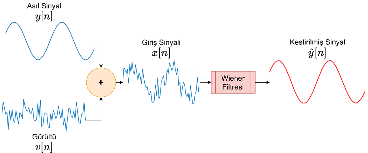
^{Figure 1. Denoising of a one-dimensional signal using the Wiener Filter}

The Wiener filter is a linear and time-invariant filter used to estimate the original form of a noisy or time-shifted signal. Therefore, although referred to as a filter, it can also be used for prediction. In the design of the Wiener filter, the following properties are assumed for the input signal $x[n]$.

1. $x[n]$ is wide-sense stationary, meaning its variance and expected value are constant and finite, and its autocorrelation function depends only on the time lag.
2. The expected value of all signals (input, output, and noise) is zero.

The Wiener filter can be designed in different categories: continuous-time versus discrete-time, and causal versus non-causal.

The Wiener Filter was developed by Norbert Wiener in 1942. Wiener designed this method to reduce noise in radar signals. Subsequently, the technique was adopted in electronics and other fields, and over time adapted for digital signal and image processing applications.

Applications

1. Signal Processing: Used to enhance radar and sonar signals acquired in noisy environments. For example, it is applied in submarine sonar systems for target detection.
2. Image Processing: Commonly preferred to reduce noise and reveal details in digital images (Figure 2). It is successfully used in medical imaging devices (MRI and CT).
3. Telecommunications: Preferred to reduce the error rate in data signals corrupted by noise.
4. Audio Processing: Applied to improve noisy audio recordings and enhance their intelligibility.

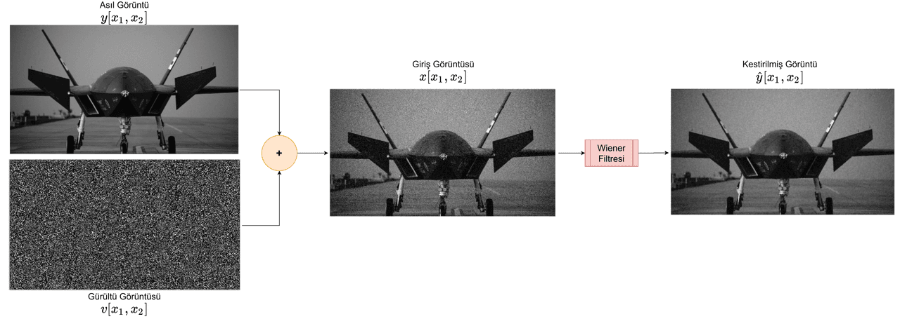
^{Figure 2. Result of image processing using the Wiener Filter}

The system representation is shown in Figure 3. Here, the signal $y[n]$ represents the desired output, while $\hat{y}[n]$ denotes the estimated signal. $x[n]$ represents the input signal. The MSE is defined as:

$MSE=E[e^2[n]]=E[(\hat{y}[n]-y[n]{)}^2]=E[{\hat{y}}^2[n]]-2E[y[n]\hat{y}[n]]+E[y^2[n]]={\Phi }_{\hat{y}\hat{y}}[0]-2{\Phi }_{y\hat{y}}[0]+{\Phi }_{yy}[0]$

$E[\cdot ]$ is the expected value operator, ${\Phi }_{\hat{y}\hat{y}}$ and ${\Phi }_{yy}$ are autocorrelation functions, and ${\Phi }_{y\hat{y}}$ is the cross-correlation function. As shown in Figure 3, the signal $\hat{y}[n]$ is produced by passing the input signal $x[n]$ through the system $h[n]$. This operation is expressed in the discrete-time domain as convolution:

$\hat{y}[n]=\sum _{m=-\infty }^{\infty }h[m]x[n-m]$

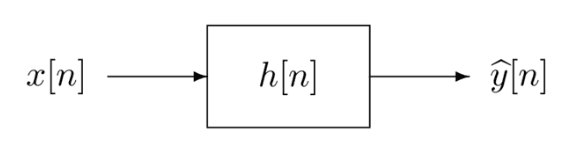
^{Figure 3:  Linear Time Invariant (LTI), discrete-time, non-causal Wiener filter,} $h[n]$^.

Based on this information, the autocorrelation and cross-correlation values forming the MSE are computed as follows:

${\Phi }_{y\hat{y}}[0]=E[y[n]\hat{y}[n]]=E[\sum _{m=-\infty }^{\infty }h[m]x[n-m]y[n]]=\sum _{m=-\infty }^{\infty }h[m]{\Phi }_{xy}[m]$

${\Phi }_{\hat{y}\hat{y}}[0]=[\hat{y}[n]\hat{y}[n]]=E[\sum _{m=-\infty }^{\infty }h[m]x[n-m]\sum _{l=-\infty }^{\infty }h[l]x[n-l]]=\sum _{m=-\infty }^{\infty }\sum _{l=-\infty }^{\infty }h[m]h[l]{\Phi }_{xx}[l-m]$

Substituting the computed autocorrelation and cross-correlation values, the MSE is rewritten as:

$MSE={\Phi }_{yy}[0]-2\sum _{m=-\infty }^{\infty }h[m]{\Phi }_{xy}[m]+\sum _{m=-\infty }^{\infty }\sum _{l=-\infty }^{\infty }h[m]h[l]{\Phi }_{xx}[l-m]$

We now take the first and second derivatives of MSE with respect to the system $h$:

$\frac{dMSE}{dh[n_i]}=-2{\Phi }_{xy}\left[n_i\right]+2\sum _{m=-\infty }^{\infty }h[m]{\Phi }_{xx}[n_i-m]$

$\frac{d^2\mathrm{MSE}}{dh[n_i{]}^2}=2{\Phi }_{xx}[0]$

${\Phi }_{xx}[0]=E[x^2[n]]$ is the autocorrelation function, which, as observed, is in quadratic form and therefore always non-negative. Consequently, MSE is a convex function. Since MSE is convex, the point where its derivative equals zero corresponds to the minimum MSE. Using this property, the minimum MSE condition is derived as:

$-2{\Phi }_{xy}[n_i]+2{\sum }_{m=-\infty }^{\infty }h[m]{\Phi }_{xx}[n_i-m]=0,\forall n_i$

$\sum _{m=-\infty }^{\infty }h[m]{\Phi }_{xx}[n_i-m]={\Phi }_{xy}[n]$

The above equation can be written in closed form using the convolution operator:

$h[n]\ast {\Phi }_{xx}[n]={\Phi }_{xy}[n]$

For convenience, we transform into the z-domain. The Z-transforms of the correlation functions in the time domain yield the spectral power functions, $S(\cdot )$.

$H(z)S_{xx}(z)=S_{xy}(z)$

$H(z)=S_{xy}(z)S_{xx}^{-1}(z)$

Thus, the general Wiener filter is designed. The Wiener filter can also be expressed in the Laplace domain:

$H(s)=S_{xy}(s)S_{xx}^{-1}(s)$

Thus, filters designed in the Laplace and z-domains can be transformed back into continuous-time and discrete-time domains respectively.

Example

_{Figure 4: Linear Time Invariant (LTI), discrete-time, non-causal Wiener filter example. All signals are wide-sense stationary and there is no correlation between signal} $y[n]$ _{and noise} $v[n]$_.

In the example shown in Figure 4, there is no correlation between $y[n]$ and $v[n]$, and all signals are wide-sense stationary (WSS), with $h[n]$ being the Wiener filter. As previously derived, the Wiener filter in the z-domain is:

$H(z)=S_{xy}(z)S_{xx}^{-1}(z)$. The functions $S_{xy}(z)$ and $S_{xx}^{-1}(z)$ are computed as follows:

${\Phi }_{xx}[k]=E[x[n]x[n+k]]$

$=E\left[\right(y[n]+v[n]\left)\right(y[n+k]+v[n+k]\left)\right]$

$=E[y[n]y[n+k]]+E[y[n]v[n+k]]+E[v[n]y[n+k]]+E[v[n]v[n+k]]$

$={\Phi }_{yy}[k]+0+0+{\Phi }_{vv}[k]$

$S_{xx}(z)=S_{yy}(z)+S_{vv}(z)$

${\Phi }_{xy}[k]=E[x[n]y[n+k]]$

$=E\left[\right(y[n]+v[n])y[n+k]]=E[y[n]y[n+k]]+E[v[n]y[n+k]]$

$={\Phi }_{yy}[k]+0$

$S_{xy}(z)=S_{yy}(z)$

Thus, the Wiener filter is obtained as:

$H(z)=S_{xy}(z)S_{xx}^{-1}(z)=\frac{S_{yy}(z)}{S_{yy}(z)+S_{vv}(z)}$

It optimizes a noisy signal or image by using the power spectral densities of both the input signal and the noise. The Wiener filter preserves the signal at frequencies with high signal-to-noise ratio (SNR) and suppresses noise at frequencies with low SNR.

The approach developed by Shannon and Bode can be used for causal Wiener filter design:

1. The input signal’s autocorrelation is computed, and its stable poles and zeros, ${\Phi }_{xx}^{++}[k]$, are separated from its unstable poles and zeros, ${\Phi }_{xx}^{--}[k]$.
2. ${\Phi }_{xx}^{++}[k]$ and ${\Phi }_{xx}^{--}[k]$ are transformed into the z-domain or Laplace domain as $S_{xx}^{++}$ and $S_{xx}^{--}$ respectively.
3. The inverse of the stable system is taken, $\frac{1}{S_{xx}^{++}(z)}$, yielding a whitening filter.
4. A new filter is constructed using the unstable system: $\hat{h}=\frac{S_{xy}(z)}{S_{xx}^{--}(z)}$.
5. $\hat{h}$ is transformed into the time domain, and its stable components are isolated. The stable portion is then transformed back into the z-domain or Laplace domain: $\hat{h}=\frac{S_{xy}(z)}{S_{xx}^{--}(z)}$.
6. The causal Wiener filter is obtained as: ${\hat{h}}^{+}=\frac{1}{S_{xx}^{++}(z)}{\left[\frac{S_{xy}(z)}{S_{xx}^{--}(z)}\right]}^{+}$.

Advantages:

- Provides the optimal result in terms of minimum mean squared error (MSE).

- Can be applied in both analog and digital systems.

- Achieves high success rates when the noise level and the power spectral densities of the signal are known in advance.

Limitations:

- Requires complete knowledge of the statistical properties of the signal and noise.

- Incorrect estimation of the power spectral densities may lead to faulty filtering.

- High computational complexity may increase processing load in real-time applications.

The Wiener filter can be implemented in both the time and frequency domains. Frequency domain implementation is typically performed using the Fast Fourier Transform (FFT). The mathematical steps are as follows:

1. Compute the Fourier transform of the noisy signal.
2. Apply weighting using the Wiener filter.
3. Perform the inverse Fourier transform to return to the time domain.

As an example, for removing salt-and-pepper noise from an image, the following steps are followed:

1. Compute the power spectrum of the noisy image.
2. Estimate the power spectral density of the noise.
3. Apply the Wiener filter to optimize the image.

The Wiener filter is becoming more flexible and dynamic through integration with emerging artificial intelligence and machine learning techniques. In particular, adaptive filtering methods build upon the Wiener filter by learning signal and noise characteristics in real time for optimization. These advancements offer broader application potential in fields such as medicine, autonomous vehicles, and space technology.